
Introduction
In July 2007, the Queensland state government in Australia introduced a new graduated driver licensing process. The new policy increased restrictions on new drivers, including a 100-hour supervised driving requirement, in addition to passenger limits, certain vehicle usage, and cell phone use. The aim of the policy change was to reduce the number of car crashes involving new drivers. A study was conducted, (Senserrick et al. Associations between graduated driver licensing and road trauma reductions in a later licensing age jurisdiction: Queensland, Australia. PLoS ONE 2018 Sep 25;13(9):e0204107), to quantify the impact of the program.
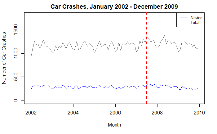
In this post, I will use a subset of the data available from this study to quantify the impact of the program using interrupted time series analysis. The data includes the monthly number of crashes for both new and total drivers, from January 2002 to December 2009.
Please find the full script and data for this post at : Github
Interrupted Time Series
A time series is simply a data set that includes some metric measured at regular time intervals. In this example, the time series I am analyzing measures the both the new and total number of monthly car crashes in Queensland. An interrupted time series (ITS) analysis aims to quantify the impact of an intervention on the measurement. To do this, the period before and after the intervention are included, and the effects of the intervention are evaluated by changes in the level and slope of the time series. Similar to my posts on causal inference, ITS is a form of a quasi-experimental study where observational data is used to evaluate the effectiveness or impact of an intervention.
In this post, I will be use a segmented regression approach for my analysis. Other time series models can be used, such as ARIMA models, but a segmented regression is simpler and more interpretable, and models the data well in this context. A segmented regression partitions the independent variable, in this case car crashes, into intervals and fits a separate linear model to each segment. The level and slope change can then be compared to assess the intervention effect.
Fitting a Segmented Regression Model
Before fitting a model, let’s quickly look at the time series plot. Overall, the observations seem relatively flat over the entire timeframe. There are local maxima and minima throughout the series, as spikes occur month to month. I do notice that the intervention occurs during a positive trend for both total and novice crashes. Also, upon observation, it does seem that the novice crashes begin to decrease following the intervention, which I will explore further.
When working with time series, there are certain assumptions that need to be accounted for when creating the models. Namely, autocorrelation usually exists, which is the correlation between observations, usually a function of the time lag between the observations. Also, seasonality is usually an issue as well. There are a number of ways to identify and measure these assumptions, such as seasonal plots, decomposition plots, ACF plots, and the Ljung-Box test for autocorrelation.I won’t include each of these in this post. Please refer to the Github script to see this code.
To set up the data for the segmented regression, the following vectors must be created : (1) A sequential time vector to track the time periods for duration of the pre and post intervention study. (2) Indicator vector to indicate pre and post intervention, both for immediate and one month lag. (3) A sequential time vector to track the time periods for duration of only the post intervention, also with the one month lag. (4) The seasonal dummy variable
A one month lag is included since the effect of the intervention may be delayed. This is a subjective decision, and analysts must decide what sort of lag to include when performing these analysis because the result will be different. A seasonal dummy variable is also included to control for the monthly seasonality present in car crashes. Please refer to the Github script to see this code.
A variety of segmented regression models were fit and compared, which differed on their use of the lagged time vector and monthly dummy variable. To compare the models, residual plots, AIC, and autocorrelation tests were examined. The final model chosen, shown below, did not include the lagged time variable and did include the monthly dummy variable. The summary output and 95% confidence intervals for the parameters are displayed.
##
## Call:
## lm(formula = novice_ts ~ time + grad + time.after + month)
##
## Residuals:
##     Min      1Q  Median      3Q     Max
## -37.907 -12.283   0.872  11.114  34.212
##
## Coefficients:
##             Estimate Std. Error t value Pr(>|t|)
## (Intercept) 288.3861     7.6445  37.725  < 2e-16 ***
## time         -0.0933     0.1155  -0.808 0.421449
## grad         56.2196     8.0314   7.000 6.74e-10 ***
## time.after   -3.5082     0.3946  -8.890 1.31e-13 ***
## monthJan    -35.0275     8.9522  -3.913 0.000189 ***
## monthFeb    -17.6822     8.9429  -1.977 0.051419 .
## monthMar     16.2882     8.9355   1.823 0.072016 .
## monthApr      1.1335     8.9300   0.127 0.899308
## monthMay      3.2289     8.9263   0.362 0.718500
## monthJun     -3.0508     8.9245  -0.342 0.733353
## monthJul      6.2056     8.9456   0.694 0.489849
## monthAug     14.8645     8.9328   1.664 0.099967 .
## monthSep    -10.7266     8.9228  -1.202 0.232802
## monthOct      7.8072     8.9156   0.876 0.383791
## monthNov     17.3411     8.9113   1.946 0.055127 .
## ---
## Signif. codes:  0 '***' 0.001 '**' 0.01 '*' 0.05 '.' 0.1 ' ' 1
##
## Residual standard error: 17.82 on 81 degrees of freedom
## Multiple R-squared:  0.6523, Adjusted R-squared:  0.5922
## F-statistic: 10.86 on 14 and 81 DF,  p-value: 2.186e-13

##                   2.5 %      97.5 %
## (Intercept) 273.1760123 303.5961844
## time         -0.3230393   0.1364428
## grad         40.2397220  72.1994777
## time.after   -4.2933830  -2.7230155
## monthJan    -52.8395840 -17.2154714
## monthFeb    -35.4758444   0.1114851
## monthMar     -1.4907773  34.0671140
## monthApr    -16.6343919  18.9014246
## monthMay    -14.5316950  20.9894238
## monthJun    -20.8076911  14.7061160
## monthJul    -11.5932712  24.0045420
## monthAug     -2.9088584  32.6378750
## monthSep    -28.4800956   7.0268581
## monthOct     -9.9320020  25.5465103
## monthNov     -0.3895912  35.0718454
From this output, I can observe the impact of the intervention on novice crashes. The 95% confidence intervals for grad (the step) and time.after (slope) are (40.2, 72.2) and (-4.3,-2.7) respectively. Therefore, there was a positive step change but a negative slope change for the period following the intervention.
The grad estimate shows that immediately after the intervention went into effect, the novice crashes had an increased level shift in monthly crashes estimated between 40 and 72. Therefore the intervention was associated with an immediate increase in monthly novice crashes. However, it is important to notice that the novice crashes were rising before the intervention and reached a maximum around the beginning of 2008 from the decomposition plot. It is reasonable that this step might be due something else occurring at the time. Also, the intervention most likely had a delayed effect due to people understanding and using the new system. Behavior change can take a while to permeate, even when laws are put into place. A more in-depth analysis using a larger lag period (6 months) would be useful in this situation.
However, the time.after estimate shows that the monthly novice crashes had a negative trend between 2.7 and 4.3 crashes a month for the duration of the study period. This indicates that while the immediate effect increased the crashes, the crashes began to decrease as the duration of the intervention increased. It simply might have taken a long time for the intervention and rules to translate to different actions being taken by drivers.
Counterfactual
To assess whether the intervention actually caused the changes, a counterfactual or negative control series can be used. A negative control series for this example would be the monthly crash data for novice drivers from another state where the intervention was not put in place. The ideal negative control series would be a similar population to the NSW novice drivers, so novice drivers from another state would have similar baseline characteristics (years of driving experience, age, gender, socio-economic status, etc). By using a similar population, certain confounding variables effects on the outcome can be controlled for. This helps me make a causal inference about the true effect of the intervention on crashes. If I saw a similar pattern in the negative control series (positive step and negative slope), then I would assume that something else besides the intervention was causing this effect. If the pattern had no change or was different in the negative control series, that would add more proof that there was a causal effect on crashes due to the intervention. In this case, I was not able to find a suitable dataset to perform this part of the analysis.
Summary
Interrupted Time Series Analysis is a powerful tool for any analyst working in healthcare. New programs and interventions are being launched all the time in the healthcare setting, and this is one very useful tool to properly evaluate the effectiveness of these programs. I hope this post can give readers a starting point in implementing these sort of analysis in their workplace. As always, please reach and connect if this topic interests you!