Introduction
Childhood growth is monitored during infancy to understand growth trajectories and identify health issues. It is also important to recognize other factors that might be impacting a child’s growth trajectory.
In this post, I am going to explore children’s weight change over time. I will use a multilevel model approach to model the change. I will also explore other factors, such as environmental and health, that may have an impact on weight change and thus improve the model. I will utilize data that incorporates maternal and family demographics, as well as child birth outcomes. The data is from the National Children’s Study Archive. The National Children’s Study (NCS) collected birth and early childhood data on more than 5,000 children and their families in the USA from 2009-2014.
Multilevel Models
Multilevel models (also known by hierarchical linear models, mixed models, or random effect models to name a few) are statistical regression models where certain parameters vary at one or more levels. For example, you can think about patients as one level, groups of patients within a diagnosis group as another level, and finally the hospital as another level. By using multilevel models, questions can be asked not just about the lowest level or individual, but also about the hierarchical levels and the interactions, or effects, between the higher and lower levels.
In this post, I will be using what is a called a longitudinal multilevel model. In this case, repeat measurements for weight are taken over a child’s first 24 months of life at 6 month intervals. In the context of the levels above, the child is the level two variable and the weight during each visit is the level one variable. In multilevel models, random intercepts and slopes can be used to examine the differences in both the intercept and slope for groups, or levels.
In this case, the variable visit (age in months) will be modeled as a random effect. This is due to the assumption that a subject’s visit will have an effect on their weight. Children will experience varying weight patterns at differing ages, so visit will need to be modeled as a random variable to account for this. If visit was not modeled as a random effect, each subject would experience the same slope, or weight over time. By adding visit as a random effect, this slope can differ between subjects and properly account for the varying weight patterns.
This is a cursory introduction to multilevel models, and I would highly recommend reading more if you are interested! Below, I will create a simple multilevel model and interpret the results!
Creating a Model
First, let’s take a look at a scatterplot to visualize the weight gain between the different genders as an example :
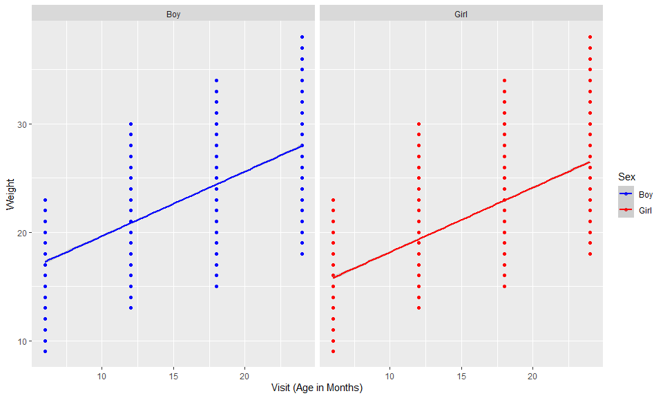
Using this example, you can observe that the intercept for boys appears to be higher than girls, while the slope (or weight over time) appears about the same. In the following models, I will explore both a random intercept and slope model. I will also add a few covariates into the model to hopefully improve the model performance.
First, the code below fits a simple random intercept (or variance-component) model. This model allows each child (level 2 variable) to have a different intercept.
#variance-component model
rand_int <- lme(visit_wt ~ 1, data = child, random = ~1|child_pidx, method="ML",control = list(opt="optim"))
summary(rand_int)
## Linear mixed-effects model fit by maximum likelihood
##  Data: child
##        AIC   BIC    logLik
##   62501.29 62523 -31247.64
##
## Random effects:
##  Formula: ~1 | child_pidx
##         (Intercept) Residual
## StdDev:    1.197309 4.947873
##
## Fixed effects: visit_wt ~ 1
##                Value  Std.Error   DF  t-value p-value
## (Intercept) 22.08322 0.05271878 5995 418.8871       0
##
## Standardized Within-Group Residuals:
##          Min           Q1          Med           Q3          Max
## -2.573897340 -0.706246867 -0.008832508  0.655650781  3.124198471
##
## Number of Observations: 10262
## Number of Groups: 4267
Above, I observe the intercept value of 22.1. This is equivalent to the mean weight for all children and all visits. I also I observe a standard deviation of basically zero for the intercept between the different subjects. So there really isn’t much variability in the beginning weight between subjects. This tells me that a hierarchical model isn’t really needed to examine the random intercept effect.
Below, I will fit a random slope model to further examine the effect of time on weight between the subjects. To do this, the slope of the relationship is allowed to vary between children.
#longitudinal multilevel linear model with random slope
rand_slope <- lme(visit_wt ~ visit, data = child, random = ~1+visit|child_pidx, method="ML",control = list(opt="optim"))
summary(rand_slope)
## Linear mixed-effects model fit by maximum likelihood
##  Data: child
##        AIC     BIC    logLik
##   50696.18 50739.6 -25342.09
##
## Random effects:
##  Formula: ~1 + visit | child_pidx
##  Structure: General positive-definite, Log-Cholesky parametrization
##             StdDev    Corr
## (Intercept) 1.7319645 (Intr)
## visit       0.1248351 -0.041
## Residual    2.0397584
##
## Fixed effects: visit_wt ~ visit
##                 Value  Std.Error   DF  t-value p-value
## (Intercept) 12.825977 0.06366397 5994 201.4637       0
## visit        0.609103 0.00412406 5994 147.6950       0
##  Correlation:
##       (Intr)
## visit -0.748
##
## Standardized Within-Group Residuals:
##         Min          Q1         Med          Q3         Max
## -3.90436717 -0.49754368 -0.02999834  0.46115135  4.74646408
##
## Number of Observations: 10262
## Number of Groups: 4267
From the longitudinal multilevel linear model output above, I observe that with visit introduced as a predictor, the intercept and standard deviation of weight between children changes. The visit variable is significant, and has a regression coefficient of 0.6, which indicates a positive relationship with weight. As expected, weight increases at visit increase. I also observe more significant standard deviations for the intercept and visit, values of 1.7 and 0.1 respectively. These values indicate that a random intercept and slope model is needed.
From the model with visit added as a random slope, I observe a -0.8 correlation which indicates a negative covariance between the random intercept and the random slope. This indicates that children with higher random intercepts were more likely to have a less positive association between weight and visit (lower random slope). Simply put, children with a higher initial weight experienced less increase in weight as age progressed.
Now that I have fit a simple random intercept and slope model, I can expand on the model by adding in non-linear time covariates (a growth curve model) or additional covariates to improve model fit. In this post, I will add a couple of covarietes to measure the improvement of the model and examine their respective effects on weight gain in children. Usually, I would conduct a thorough exploratory data analysis at the beginning to study relationships in the data and make hypothesis about which variables might influence weight. However, for the purpose of this post, I am just choosing three covariates (child health at visit, sex, and household income) to examine. The code for fitting this model is below.
#longitudinal multilevel linear model with fixed covariates
cov_model <- lme(visit_wt ~ visit + child_health + child_sex + household_income, data = child, random = ~1+visit|child_pidx, method="ML",control = list(opt="optim"))
summary(cov_model)
## Linear mixed-effects model fit by maximum likelihood
##  Data: child
##        AIC      BIC    logLik
##   50364.06 50429.19 -25173.03
##
## Random effects:
##  Formula: ~1 + visit | child_pidx
##  Structure: General positive-definite, Log-Cholesky parametrization
##             StdDev    Corr
## (Intercept) 1.5314920 (Intr)
## visit       0.1234441 -0.019
## Residual    2.0432317
##
## Fixed effects: visit_wt ~ visit + child_health + child_sex + household_income
##                      Value  Std.Error   DF   t-value p-value
## (Intercept)      13.875876 0.13635114 5993 101.76575  0.0000
## visit             0.609394 0.00409728 5993 148.73154  0.0000
## child_health     -0.073284 0.05453291 5993  -1.34385  0.1790
## child_sexGirl    -1.505892 0.08101657 4264 -18.58745  0.0000
## household_income -0.095161 0.03650794 4264  -2.60657  0.0092
##  Correlation:
##                  (Intr) visit  chld_h chld_G
## visit            -0.347
## child_health     -0.602  0.031
## child_sexGirl    -0.317  0.006  0.039
## household_income -0.624 -0.027  0.064  0.000
##
## Standardized Within-Group Residuals:
##         Min          Q1         Med          Q3         Max
## -3.96141584 -0.49735755 -0.02637587  0.47061957  4.65021609
##
## Number of Observations: 10262
## Number of Groups: 4267
From the model output above, I observe that child_sex and household_income are significant predictors, while child_health is not significant. The visit variable still has a coefficient of 0.66. The child_sex variable (SexGirl) has a coefficient of -1.5, which can be interpreted as girl’s weight measurement being 1.5 less on average when compared to the baseline (male) weight values. The household_income has a coefficient of -0.1, which can be interpreted as a negative association with household income. As household income rises (based on category), the weight values decrease.
Summary
In this post, I explained what multilevel models are and went through a simple model fitting exercise to illustrate a use case. I hope you were able to appreciate the value of multilevel models, especially in answering more complex questions in our data. From this example, I was able to move beyond a simple statistical question like how does weight differ between genders in early childhoold to how does household income impact weight gain in children over time. As a practicing health data scientist, these questions arise frequently and multilevel models are a great tool to know. I hope you enjoyed this brief introduction, and please reach out!