Introduction
Young maternal age is associated with adverse pregnancy outcomes, including low birthweight and preterm birth. However, arguments have been made that young maternal age is not actually causing these outcomes. Instead, other socio-economic factors associated with young maternal age actually lead to these adverse outcomes.
In this post, I will explore the causal relationships further to hopefully shed light on the question above. I will utilize data that incorporates maternal and family demographics, as well as child birth outcomes. The data is from the National Children’s Study Archive. The National Children’s Study (NCS) collected birth and early childhood data on more than 5,000 children and their families in the USA from 2009-2014.
Directed Acyclic Graphs
Directed Acyclic Graphs (DAGs) are used by epidemiologists to help determine the unbiased estimate of effect of an exposure on an outcome. In other words, DAGs are used to make causal inferences about the exposure. To create a DAG, a researcher visualizes their assumptions about the causal relationships between variables present in the data. Once the causal structure present in the data is visualized in a DAG, it is easier to explore confounding relationships and properly control on certain variables in order to make causal inferences about the exposure of interest. If you are interested in more information about DAGs and causal relationships, this resource might be helpful.
In this case, I am interested in estimating the effect of young maternal age on preterm birth. I include a number of socio-economic factors and maternal demographics to complete the analysis. Below, the DAG for this analysis is pictured. Note, I am not working with any subject matter experts on this post so many of my assumptions might be inaccurate.
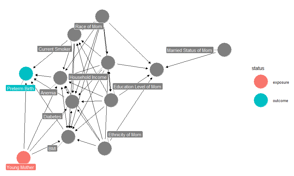
The DAG is very busy, but it can be useful to map paths between exposure and outcome. For this analysis, I am interested in controlling for “backdoor” paths. These are variables that affect both the exposure (Young Mother) and outcome (PreTerm Birth). I observe a few backdoor paths:
-
Young Mother <– Race of Mom –> (BMI,Diabetes,Anemia,Current Smoker) –> PreTerm Birth
-
Young Mother <– Education Level of Mom –> (BMI,Diabetes,Anemia,Current Smoker) –> PreTerm Birth
-
Young Mother <– Household Income –> (BMI,Diabetes,Anemia,Current Smoker) –> PreTerm Birth
-
Young Mother <– Ethnicity of Mom –> (BMI,Diabetes,Anemia,Current Smoker) –> PreTerm Birth
From above, Race, Education Level, Ethnicity, and Household income will need to be controlled for in order to properly make causual inferences about the effect of young maternal age on preterm birth. There are a variety ways to do this, but I will explain the matching method below.
Matching
In a perfect world, randomized-control trials (RCTs) are used to explore unbiased estimates of exposure effects. RCTs lead to unbiased estimates by randomly assigning subjects to either the control or exposure group, thus limited the bias present in the subject’s backgrounds and characteristics. RCTs are not always perfect, but if proper techniques are used to choose the sample and assign to the groups, they are the gold standard of clinical research.
However, RCTs can be difficult and sometimes impossible to implement in real life. In this example, there is simply no way to create a RCT where some mothers give birth early and some mothers give birth later in the proper way. So, what to do? Enter Matching!
Matching is a technique that balances certain characteristics in the groups of interest (control vs exposure) to limit the confounding effect of these variables on the exposure and outcome. There are a variety of methods to perform matching, but the details are out of scope for this post. At its core, matching algorithms seek to find a similar control subject for every exposure subject. Similar here is defined by the researcher. In this case, I want to control for race, education level, ethnicity, and household income. Therefore, for every young mother, I want to find a normal mother with similar race, education level, ethnicity, and household income characteristics. The former statement is possible by using “exact” matching, that is, matching subjects with exact variables. However, propensity score matching is used in this instance. This leads to subjects with a similar propensity score, however, it does not necessarily mean that the variables are exact. This is a limitation of propensity score matching, but I will still be using this method in this case.
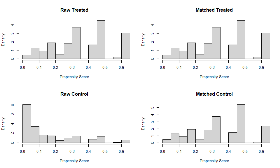
Below, you can observe the difference in the means between the treated and control groups for all the data, and for the matched data. You also can see the propensity score distribution for the raw data and matched data. Here, the propensity score reflects the matching method used. As you can see, the matched data’s background characteristics are more balanced when compared to the raw data. This can be observed in the identical means and near identical distributions of propensity scores.
##
## Call:
## matchit(formula = young_mom ~ mom_race + mom_education + household_income +
##     mom_ethnicity, data = child, method = "nearest", distance = "logit",
##     discard = "none", ratio = 1)
##
## Summary of balance for all data:
##                  Means Treated Means Control SD Control Mean Diff eQQ Med
## distance                0.3616        0.1474     0.1632    0.2142  0.2461
## mom_race                1.9557        1.6916     1.3337    0.2641  0.0000
## mom_education           2.2299        3.9232     1.6131   -1.6933  2.0000
## household_income        1.3213        2.3385     1.0984   -1.0171  1.0000
## mom_ethnicity           1.7673        1.8298     0.3759   -0.0625  0.0000
##                  eQQ Mean eQQ Max
## distance           0.2142  0.3396
## mom_race           0.2632  2.0000
## mom_education      1.6911  3.0000
## household_income   1.0166  2.0000
## mom_ethnicity      0.0623  1.0000
##
##
## Summary of balance for matched data:
##                  Means Treated Means Control SD Control Mean Diff eQQ Med
## distance                0.3616        0.3559     0.1626    0.0057       0
## mom_race                1.9557        1.9127     1.4061    0.0429       0
## mom_education           2.2299        2.2341     1.0330   -0.0042       0
## household_income        1.3213        1.3144     0.6316    0.0069       0
## mom_ethnicity           1.7673        1.7285     0.4450    0.0388       0
##                  eQQ Mean eQQ Max
## distance           0.0058   0.141
## mom_race           0.0512   1.000
## mom_education      0.0042   1.000
## household_income   0.0069   1.000
## mom_ethnicity      0.0388   1.000
##
## Percent Balance Improvement:
##                  Mean Diff. eQQ Med eQQ Mean eQQ Max
## distance            97.3240     100  97.2808 58.4927
## mom_race            83.7399       0  80.5263 50.0000
## mom_education       99.7546     100  99.7543 66.6667
## household_income    99.3191     100  99.3188 50.0000
## mom_ethnicity       37.9516       0  37.7778  0.0000
##
## Sample sizes:
##           Control Treated
## All          3126     722
## Matched       722     722
## Unmatched    2404       0
## Discarded       0       0
Estimating the Effect
Now, I can utilize the matched dataset to create a simple logistic regression model to estimate the effect of young maternal age on preterm birth. By comparing this model to the same model using all the data, I can observe the differences and make conclusions about the unbiased exposure effect on the outcome.
Below, the output for the raw model is displayed. Note here that young maternal age is a significant predictor of preterm birth, and has a positive assocation.
##
## Call:
## glm(formula = preterm_birth ~ young_mom, family = binomial, data = child)
##
## Deviance Residuals:
##     Min       1Q   Median       3Q      Max
## -0.6328  -0.5549  -0.5549  -0.5549   1.9734
##
## Coefficients:
##             Estimate Std. Error z value Pr(>|z|)
## (Intercept) -1.79325    0.05114 -35.066  < 2e-16 ***
## young_mom    0.28663    0.10927   2.623  0.00871 **
## ---
## Signif. codes:  0 '***' 0.001 '**' 0.01 '*' 0.05 '.' 0.1 ' ' 1
##
## (Dispersion parameter for binomial family taken to be 1)
##
##     Null deviance: 3252.5  on 3847  degrees of freedom
## Residual deviance: 3245.8  on 3846  degrees of freedom
## AIC: 3249.8
##
## Number of Fisher Scoring iterations: 4
Below, the output for the matched model is displayed. Note here that now the young maternal age is not a significant predictor of preterm birth, and has no association.
##
## Call:
## glm(formula = preterm_birth ~ young_mom, family = binomial, data = match_data)
##
## Deviance Residuals:
##     Min       1Q   Median       3Q      Max
## -0.6408  -0.6408  -0.6328  -0.6328   1.8476
##
## Coefficients:
##             Estimate Std. Error z value Pr(>|z|)
## (Intercept) -1.47889    0.09573 -15.449   <2e-16 ***
## young_mom   -0.02773    0.13597  -0.204    0.838
## ---
## Signif. codes:  0 '***' 0.001 '**' 0.01 '*' 0.05 '.' 0.1 ' ' 1
##
## (Dispersion parameter for binomial family taken to be 1)
##
##     Null deviance: 1376.7  on 1443  degrees of freedom
## Residual deviance: 1376.6  on 1442  degrees of freedom
## AIC: 1380.6
##
## Number of Fisher Scoring iterations: 4
When controlling for socio-economic factors, young maternal age becomes an insignificant predictor of preterm birth. In this case, other external factors play a more significant factor in causing preterm birth. When using the matching method to properly control for confounding variables, a more unbiased estimate of the effect of young maternal age on preterm birth was able to quantified.
Summary
Casual inference is an important tool for a health data scientist to have in their toolkit. It is clear to see how improper techniques can lead to incorrect conclusions from the above example. In this post, I highlighted a few techniques that data scientists, especially in healthcare, can utilize to properly explore the casual relationships in their data. Please keep an eye out for further posts on this subject in the future. And as always, reach out if you have any questions!