
In this post, I will be conducting analysis on colon cancer survival. The dataset include information from a clinical trial on the effectiveness of two different types of chemotherapy (levamisole and levamisole+5-fluorouracil) compared to controls (i.e. no chemotherapy treatment) on survival from stage B/C colon cancer.
I will highlight the process and some key findings from the overall analysis. The complete code and analysis can be found on my Github.
Initial Survival Curves
The documentation for the dataset can be found here. This analysis will study the effects of the chemotherapy treatments as well as other clinical variables concerning the colon cancer diagnosis. The survival object for this analysis is Time and Status. Time represents the days until death or censoring. Status represents whether the individual died or whether the individual was censored. In this context, censored means the patient was still alive when the study observation took place.
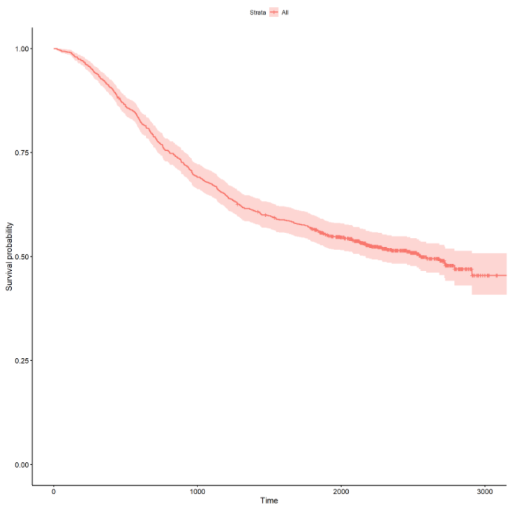
First, let’s take a look at the overall survival curve by fitting a Kaplan-Meier survival curve :
Let’s also stratify the survival curve by the treatment (rx) and more than 4 positive lymph nodes (node4) :
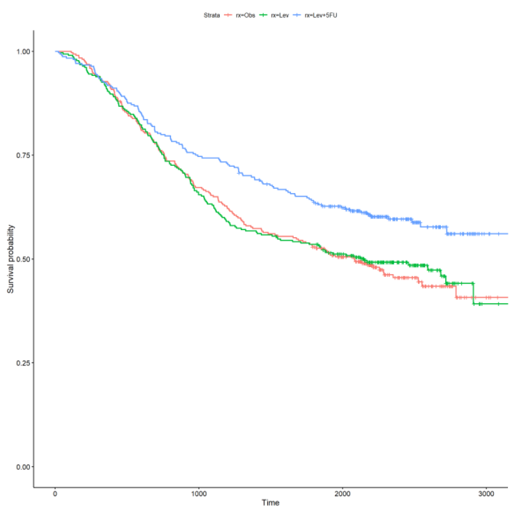
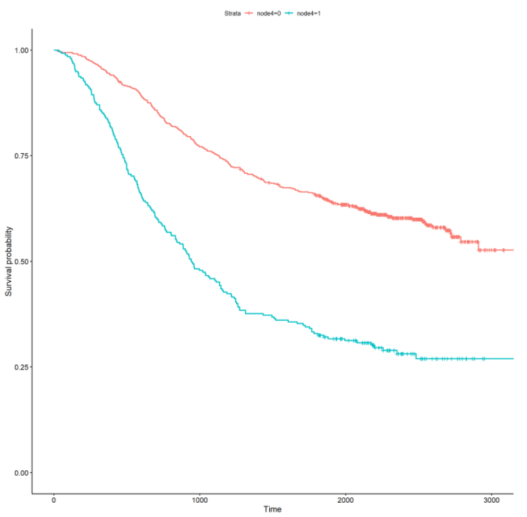
From the above curves, there is a noticeable effect for treatment and more than 4 positive lymph nodes. In the rx curve, the levamisole+5-fluorouracil treatment appears to have a positive impact on increasing survival time. From the node4 curve, patients with more than 4 positive lymph nodes appear to have a significantly decreased survival time. Survival curves stratified by categorical variables can offer initial insights into possible effects on survival time. In the next section, I will formally fit univariate and multivariate survival models to ascertain the significance and magnitude of these effects.
Fitting Survival Models
The next step in survival analysis involves fitting univariate Cox proportional hazards models (link). These models can be used to estimate the significance and effect of each invidiual predictor on the overall survival time. I don’t share the output below, but I observe that rx, obstruct, adhere, differ, extent, surg, and node4 are all statistically significant. Each variable has a statistically significant difference in the survival time between the groups.
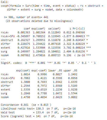
Using these variables, I can then fit a multivariate Cox model. The output summary is shown below :
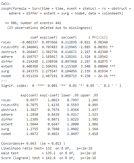
From the summary, I observe that adhere is not statistically significant anymore. Further, only the rxLev+5Fu level is statistically significant, whereas the rxLev level is not statistically significant when compared with the base level of Obs. The exponential coefficient (or hazard ratio) for rxLev+5Fu of .71 can be interpreted as reducing the hazard by a factor of .7 (or 30%) when keeping all other covariates constant. Similarly, I observe that extent and node4 have hazard ratios of 1.5 and 2.5 respectively, indicating a increased risk of death.
To further simplify the model, I remove adhere and re-fit a multi-variate Cox model, output summary below :
There is not much difference here, and I won’t go into the details concerning the output above. However, I am interested in knowing whether I can use the simplified model above versus the original multivariate model I built. To do this, I can perform a likelihood ratio test (using ANOVA) to test whether the models have a statistically significant different goodness of fit. This only works for comparing a subset of one model to another. I can also compute the [AIC] (https://en.wikipedia.org/wiki/Akaike_information_criterion) to compare models that aren’t necessarily subsets of each other. In this case, the AIC for the initial model was 5579 and the AIC for the subset model was 5578. The ANOVA output is below :
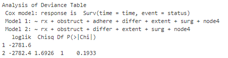
From the ANOVA output, I observe a p-value of .19, and I can conclude that I fail to reject the null hypothesis. I also observe that the AIC for the subset model is less than the AIC for the larger model, and a lower AIC is preferred. As a result, I would choose to use the subsetted model when comparing these two. If this analysis was going to be used for predictive purposes in a production setting, I might be strictly interested in predictive performance. However, if I was using this analysis to conduct research and inform policy, I might favor a simple model. In tis case, both criteria are met and the simpler model offers a similar goodness of fit.
Finally, I have to check a couple of model diagnostics to ensure that certain assumptions are met in order to use the Cox proportional hazards models. I won’t go into the detail in this post, but this involves checking the proportional hazards and linearity in the predictors. If the proportional hazards assumption is not met, the data must be cut into differing time frames and Cox models must be fit to each subset. If linearity assumption is not met, the functional form of the continous predictors must be transformed in order to continue.
Conclusion
This was my first introduction to survival analysis, and I expect to continue exploring new applications for these techniques in healthcare data. The flexibility of survival modeling is that it not only can be applied to death events, it can be applied to any time to event data. Coming from a health system operations background, I hope to work on applying these models to time to discharge (length of stay) for inpatient hospital stays in the future. Stay tuned for more!